r.stone - GRASS GIS manual

Note: This document is for an older version of GRASS GIS that has been discontinued. You should upgrade, and read the current manual page.

NAME

r.stone - The STONE rockfall module

KEYWORDS

raster, stone, rockfall

SYNOPSIS

r.stone

r.stone --help

r.stone dem=name sources=name nrest=name trest=name friction=name [stoch_funct=integer] [stoch_funct_ang=integer] ang_stoch_range=integer vrest_stoch_range=integer hrest_stoch_range=integer frict_stoch_range=integer start_vel=float stop_vel=float counter=name [maxvel=name] [maxdz=name] [--overwrite] [--help] [--verbose] [--quiet] [--ui]

Flags:

--overwrite: Allow output files to overwrite existing files
--help: Print usage summary
--verbose: Verbose module output
--quiet: Quiet module output
--ui: Force launching GUI dialog

Parameters:

dem=name [required]: Elevation raster map; The input elevation raster map
sources=name [required]: Start/stop raster map; The input start/stop integer raster file.Shows the source areas of rock fall (value > 0).Shows the areas where rock falls must stop, e.g. a lake (value = -1).
nrest=name [required]: Normal Elasticity raster map; Contains values of normal (vertical) restitution coefficient, used at impact points.Accepted values are from 0 (total energy dumping) to 100 (elastic restitution)Values are in integer percentage.
trest=name [required]: Tangential Elasticity raster map; Contains values of tangential (horizontal) restitution coefficient, used at impact points.Accepted values are from 0 (total energy dumping) to 100 (elastic restitution)Values are in integer percentage.
friction=name [required]: Friction raster map; Contains values of rolling friction angle (tan(beta)), used where rolling.Example Friction for alluvial deposit is high, beta = 40.4, tan(beta) = 0.85.Example Friction for bedrock is low, beta = 16.7, tan(beta) = 0.30
stoch_funct=integer: The stocastic simulation function to use for VElas, HElas, Frict (0 = Gaussian, 1 = Cauchy, 2 = Uniform); Default: 0
stoch_funct_ang=integer: The stocastic simulation function to use for the range of starting angles (0 = Gaussian, 1 = Cauchy, 2 = Uniform); Default: 0
ang_stoch_range=integer [required]: Percent variability of detachment angle; Default: 10
vrest_stoch_range=integer [required]: Percent variability of normal restitution; Default: 10
hrest_stoch_range=integer [required]: Percent variability of tangential restitution; Default: 10
frict_stoch_range=integer [required]: Percent variability of the friction coefficient; Default: 10
start_vel=float [required]: Start velocity; The start velocity of a rock [m/s].; Default: 1.0
stop_vel=float [required]: Stop velocity; Parameter used to define the minimum velocity for a rock fall.A velocity lower than the one specified here causes the boulder to stop. [m/s]; Default: 3.0
counter=name [required]: The resulting counters raster output map
maxvel=name: The optional maxvel raster output map
maxdz=name: The optional maxdz raster output map

DESCRIPTION
SEE ALSO
EXAMPLE
- Sample output
REFERENCES
AUTHORS

DESCRIPTION

The module r.stone is a GRASS implementation of the model STONE [1] for three-dimensional modeling of rockfall trajectories. A rockfall is a point-like block, by assumption, and the model simulates its trajectory as a sequence of falling, bouncing and rolling steps. The trajectory follows a digital elevation model, it starts from a user-defined source point(s) with a non-null initial velocity and stops downhill when all of its kinetic energy is loss (i.e., when it reaches a minimum velocity) by bouncing and/or rolling on the ground. The Coefficients of normal and tangential restitution describe the amount of kinetic energy lost in each bounce, and a friction coefficient describes the kinetic energy loss during rolling. The r.stone implementation of STONE requires a minimal set of input raster maps in addition to the DTM, including a map of sources, and three maps of numerical coefficients. The output is a raster map with values corresponding to the number of trajectories crossing each grid cell after a full simulation.

Input DTM is a square fixed spaced DTM, used as a triangular regular network built on the fly at run-time. Rockfall trajectories are evaluated using parametric second-order equations after a roto-transformation of the coordinate system to the run-time triangle. The calculation of each trajectory includes the random selection of an initial direction angle, and of cell-by-cell values of restitution and friction coefficients extracted from Gaussian distributions centered on the values specified in the corresponding input raster and limited by +/- 10% from the central value. By virtue of the random selection of initial angle and parameters, and of the possibility of simulating many trajectories from each source cell, the output assumes a probabilistic meaning.

EXAMPLE

The input parameters of r.stone listed below are all mandatory. Generating a map of source locations requires either knowledge of the area, gained through field campaigns or aerial photos, or a sound statistical method. A simplistic method to estimate the location of sources is to consider locations on steep terrain as possible rockfall sources, for example:

bash
g.region rast=dem
r.slope.aspect –e elevation=dem slope=slope
r.mapcalc “sources = if(slope>50,10,null())”

to simulate 10 trajectories originating from each cell with slope larger than 50 degrees.

Raster maps of friction and restitution coefficients can be generated based on geo-lithological knowledge of the area. Assuming a geological map, in polygonal vector format, with classes similar to the table below, we generate the input raster maps as follows:

bash
v.db.addcolumn map=geology columns='friction real, nrest integer, vrest integer'
db.execute sql=”update geology set friction=0.65 where class_id=1”
db.execute sql=”update geology set friction=0.80 where class_id=2”
...
v.to.rast input=geology use=attr attribute_column=friction output=friction

And similar operations for nrest and vrest, for all classes present in the geology map. The actual model run is as follows:

bash
r.stone dem=dem sources=sources_raster nrest=nrest_raster
        trest=trest_raster friction=friction_raster stop_vel=1
        counter=out_counter_raster

Where:

dem is the input digital elevation model.
sources is the input sources raster.
- Defines the start and stop points of the rockfalls trajectories. Positive integer values indicate source areas, while a value of -1 indicates areas where rocks must stop, such as for example a lake. Values larger than 1 trigger the simulation of a corresponding number of randomized trajectories, from the same starting point. Null cells have no effect.
nrest is the normal restitution raster map.
- Contains values of normal (vertical) restitution coefficient, useful at impact points. Accepted values are from 0 (total energy dumping) to 100 (elastic restitution). Values are expressed in integer percentage.
trest is the tangential restitution raster map.
- Contains values of tangential (horizontal) restitution coefficient, used at impact points. Accepted values are from 0 (total energy dumping) to 100 (elastic restitution). Values are expressed in integer percentage.
friction is the Friction raster map.
- Contains values of the rolling friction angle (tan(beta)).
  - Example Frictions:
  - For alluvial deposits, where the friction is high: beta = 40.4, tan(beta) = 0.85
  - For bedrock, where the friction is low: beta = 16.7, tan(beta) = 0.30
stop_vel is the parameter used to define the minimum velocity for a rock to be considered in motion. A velocity lower than the one specified here causes the boulder to stop.
counter is the output raster of the number of stones that passed through a cell.

The following table, extracted from [1], gives example values of restitution and friction coefficients corresponding to 19 lithological classes used in Italy.

Lithological class	Friction	Normal restitution	Tangential restitution
Anthropic deposits	0.65	35	55
Alluvial, lacustrine, marine, eluvial and colluvial deposits	0.80	15	40
Coastal deposits, not related to fluvial processes	0.65	35	55
Landslides	0.65	35	55
Glacial deposits	0.65	35	55
Loosely packed clastic deposits	0.35	45	55
Consolidated clastic deposits	0.40	55	65
Marl	0.40	55	65
Carbonates-siliciclastic and marl sequence	0.35	60	70
Chaotic rocks, mélange	0.35	45	55
Flysch	0.40	55	65
Carbonate Rocks	0.30	65	75
Evaporites	0.35	45	55
Pyroclastic rocks and ignimbrites	0.40	55	65
Lava and basalts	0.30	65	75
Intrusive igneous rocks	0.30	65	75
Schists	0.35	60	70
Non–schists	0.30	65	75
Lakes, glaciers	0.95	10	10

Sample output

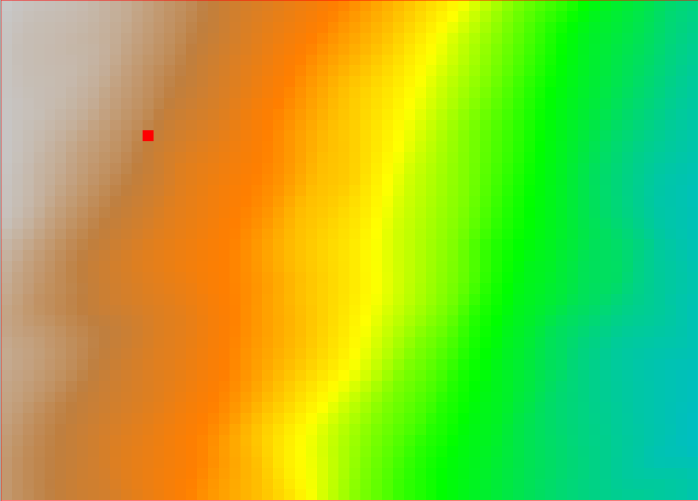
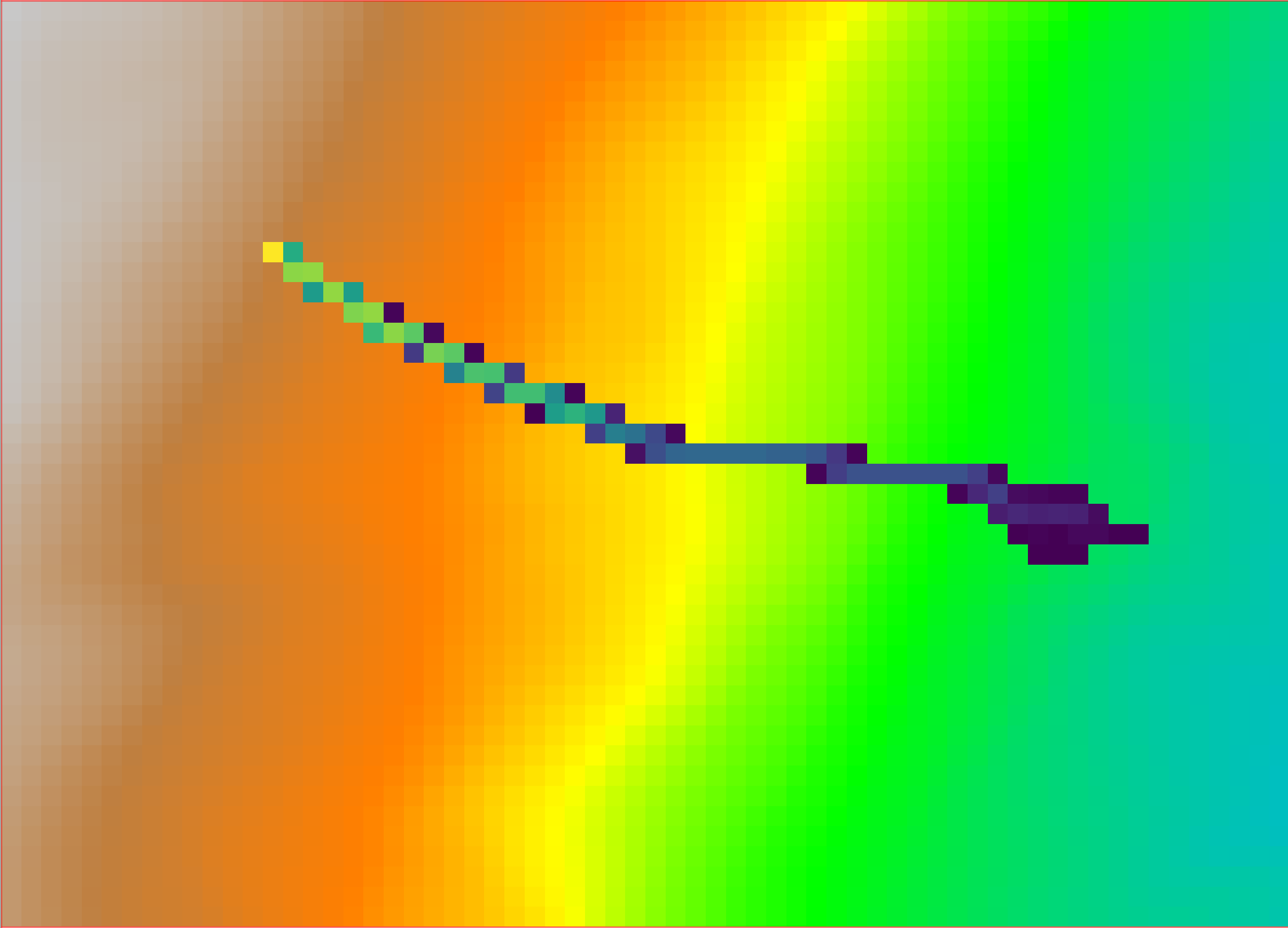
The following figures show the output of the r.stone module, initialized with an individual source point.

A sample portion of a 10m x 10m resolution DEM, with one grid cell (red square) acting as a rockfall source point, with raster value 100: the effect on the model r.stone is to simulate 100 trajectories starting from that cell.

Sample output of r.stone, depicting the counter raster map; the values of the raster output correspond to the total number of simulated trajectories going through that cell.

REFERENCES

[1] The algorithm is based on the work of Fausto Guzzetti, Giovanni Crosta, Riccardo Detti, Federico Agliardi (2002): STONE: a computer program for the three-dimensional simulation of rock-falls. Computers & Geosciences, 28(9), 1079-1093. https://doi.org/10.1016/S0098-3004(02)00025-0

[2] Example coefficients for r.stone are in: M. Alvioli et al. (2021): Rockfall susceptibility and network-ranked susceptibility along the Italian railway. Engineering Geology, 293, 106301. https://doi.org/10.1016/j.enggeo.2021.106301

AUTHORS

Fausto Guzzetti and Massimiliano Alvioli

Translation from the original code and adaptation to GRASS GIS by Andrea Antonello

SOURCE CODE

Available at: r.stone source code (history)

Latest change: Tuesday Apr 15 23:08:17 2025 in commit: c2e43d6a48ccdad264a2d10141f793b257c30e85